The research used JASP software to run the primary data collected and reported on SEM, PLS, and Bootsrap Significance. The results indicated that there is a total positive significance relationship as a total effect between work culture (independent variable) and job satisfaction (dependent variable). JASP is been named after a Bayesian pioneer called Sir Harold Jeffreys, which stands for Jeffrey’s Amazing Statistical Program. The results of the study were calculated on the following that is model fit, AIC, BIC, fit indices, other fit measures, R2, factor loadings, weights, regression coefficients, factor variance, and residual variance. This research was a quantitative study via survey in Metro Mass Transit, a population of 138 permanent drivers was the target population with a sample size of 102 using Krasjcie and Morgan's (1970) formula. This is a deductive study based on a probability sampling technique. The hypothesis was satisfied. The researcher want this research findigs to be more educative in JASP by presenting all these analysis in comparison for clear understanding and distinctions.
INTRODUCTION
This research is being derived from very wide studies of work culture and job satisfaction as the focused area. It adapted Shahin's (2016) model using two variables. The main purpose of this research is to examine and recommend best practices with clear recommendations from its findings. The goal also is to test for the total effect of the relationship between work culture (independent variable), and job satisfaction (dependent variable). By and large, the objective of this research is enormous but the general objective is to determine the common factors of work culture and job satisfaction that can help bring sustainability to the Metro Mass Transit (MMT) passenger operations (Alzain et al., 2021; Alnofaiey et al., 2022). In other words, finding out what the organization should do to bring about job satisfaction to its employees. And to achieve this, Shahin's (2016) conceptual model is adapted to distinguish it as a contribution. This is to apply quantitative research to be able to dissect the veracity of the work culture model with its relationship to job satisfaction. Perceptions of organizational justice affect work culture job attitudes and job satisfaction Wahyuhadi et al., (2023). There was a direct effect on job satisfaction and also an indirect effect on work culture (Sandika et al., 2016).
Problem Statement
Within the economy of Ghana, several reports, theories, and empirical data showed that there have been instances of staff demonstrations against the organization due to employees’ grievances about unpaid salaries and allowances. This is a result of staff dissatisfaction with their condition of service and fringed benefits. Quite often the government has removed most “Chief Executives Officers” (CEOs) of the Organisation due to the reason of malpractices and mismanagement of national resources without due diligence. These turbulent circumstances surrounding the operation of Metro Mass Transit may be due to bad work culture practices. It is argued that many studies have indicated a more complex situation on job satisfaction in motivating employees which has an impact on productivity and organizational performance (Aziri, 2011). Aziri (2011) concluded that job satisfaction has not been properly adopted by many managers of business organizations or scholars. Job satisfaction represents both negative and positive feelings that employees perceive towards their work and even though when a worker is employed in an organization, the person brings in his or her desires, needs, and experiences with the right attitude about others and the job (Ryan et al., 2017; Subramanyam & Donthu, 2022; Zayed, et al., 2022). But they can be disappointments alongside these hopes which is why there is employer-employee dissatisfaction at times.
Metro Mass Transport Limited
MMT is a transportation system of service in Ghana for the public that was set up to provide affordable and reliable transport to commuters from towns, villages, and cities in the form of intercity service movement. This was established by the Ghana government under former President John Agyekum Kufuor who conceived this idea in 2001, which was incorporated in 2003 with various shareholders. These shareholders are National Investment Bank, Ghana Oil Company, States Insurance Company (SIC), Social Security and National Insurance Trust, Agric Development Bank, and Prudential Bank Limited. All these financial institutions hold 55% of the MMT shares and the rest of the 45% is owned by the Ghana government. The slogan of the MMT is ‘moving the nation’ founded in 2003 and it provides bus rapid transit, school bus, and public bus service.
Research Questions
The following are the major research questions:
Research Objectives
This research study examines the above total effects to justify the following objective:
Hypothesis
H1: Work culture has a positive significant effect as a direct relationship to job satisfaction.
Literature Review
Job satisfaction is one of the difficult areas in today’s business and organizational management faced by managers with regard to managing employees (Aziri, 2011). Aziri (2011) argued that there is no generally accepted definition of job satisfaction and that different authors with different approaches to the term job satisfaction. Cabanas et al., (2020) defined job satisfaction as a combination of any physiological, psychological, and environmental circumstances that cause people to indicate that they are truly satisfied with their job. Although job satisfaction is influenced by many external factors it is still an internal way by which employees feel. It represents sets of factors that make employees feel satisfied (Dessler, 2015).
Ihinmoyan, (2022) defined job satisfaction regarding the employee's roles at the workplace, hence, Vroom defined job satisfaction as individual orientations that affect their work roles in a moment. Job satisfaction according to Mabaso and Dlamini (2017) defined job satisfaction as the extent to which employees are content with their reward packages out of their job in an intrinsic manner. According to Management Study Guide (2019) defined work culture as a concept that believes in the study of attitudes, thought processes, ideologies as well as principles of the organization. Work culture decides the way workers can interact with one another with regard to the functioning of the organization.
It is argued that many studies have indicated a more complex situation on job satisfaction in motivating employees which has an impact on productivity and organizational performance (Aziri, 2011). Aziri (2011) concluded that job satisfaction has not been properly adopted by many managers of business organizations or scholars. Job satisfaction represents both negative and positive feelings that employees perceive towards their work and even though when a worker is employed in an organization, the person brings in his or her desires, needs, and experiences with the right attitude about others and the job (Ryan et al., 2017; Subramanyam & Donthu, 2022; Zayed et al., 2022).
The importance of job satisfaction emerges when an employee had in mind several negative thoughts as consequences of dissatisfaction with their job such as an increase in absenteeism, lack of loyalty, increase in accidents, etc (Aziri, 2011). Dewi, (2019) argued that there are three (3) major dimensions of job satisfaction namely emotional, outcomes or exceeding expectations, and attitude of employees. Sinha et al., (2010) argued that the interest that arises in the topic of work culture in this modern times by practitioners and academicians or researchers is been caused by two factors and that is, the first assumption that organizational performance is dependent on the employees’ values are aligned to the extent of the organizations' strategy. And the second aspect is the view that work culture is subject to manipulations consciously to employees’ desired ends.
Hypothesis Development
Work Culture and Job Satisfaction
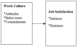
Prakoeswa et al., (2021) findings indicated that there has been a positive and significant link between job satisfaction and work culture within organizational commitment. There has been an association between work culture commitment and job satisfaction at different levels within the organization. Work culture such as personal and other job-related factors affects the job satisfaction of employees within an organization (Sandika et al., 2016). Shahin's (2016) results indicated that there have been positive influences of work culture on performance due to job satisfaction. Below is the hypothesis derived and Figures 1 and 2 as research framework and conceptual/theoretical model respectively.
H1: Work culture has a positive significant effect as a direct relationship to job satisfaction.
|
|
|
Figure 1. Research framework |
|
|
|
Figure 2. Conceptual/Theoretical Model |
MATERIALS AND METHODS
Research Design
In a way to explore the relationship between workplace culture and job satisfaction a quantitative research approach is deemed as an appropriate method design for this research.
Quantitative Research Design Technique
Quantitative research is used to quantify problems and generate numerical data that can be transformed into ideal statistics. It quantifies attitudes, opinions, behaviors, and any other defined variables, and in a way generalizes results from a larger sample population. It uses measurable data to formulate facts that uncover patterns in research. Moreover, Quantitative methods of collecting data are more highly structured than Qualitative methods of collecting data. It is a formal, objective, and systematic process for obtaining information. It is a method used to describe, test relationships and examine the cause and effects of relationships. Quantitative methods of collecting data have various forms of surveys e.g. online surveys, paper surveys, mobile surveys, face-to-face interviews, telephone interviews, kiosk surveys, systematic observations, longitudinal studies, online polls, and website interceptors (DeFranzo, 2011). This research considered a survey via the use of a questionnaire.
Population and Sampling
Metro Mass Transit Limited driver is the target population. It has the slogan “Moving the nation”. It is a Ghana government transport company that provides affordable and reliable means of transportation for the general public within towns, villages, cities, and intercity movements. It has a total population of 138 permanent drivers with a sample size of 102 using the Kresjcie and Morgan (1970) formula.
Data Collection
An extract of questionnaire results was adopted from the author’s thesis for further research on total effects.
Instruments Adopted
Job Satisfaction Instrument Developed
Agustiningsih et al., (2017) Minnesota Satisfaction Questionnaire (MSQ) distinguishes intrinsic and extrinsic factors which make it fit for this research as appropriate. This instrument has been studied, tested, and proven as reliable for the measurement of job satisfaction as Falkenburg and Schyns, (2007) obtained Cronbach alpha of 0.93 and 0.92 respectively when they used the same questionnaire in similar research studies from two different organizations. Elangovan's (2001) study of job satisfaction and the results of the reliability analysis was Cronbach alpha of 0.89. Wahyuhadi et al., (2023) researched social bonding theory and the Cronbach alpha was 0.89. Udechukwu (2007) studied job satisfaction in correctional settings and the results of Cronbach alpha of 0.88. A study by Wahyuhadi et al., (2023) on job satisfaction among academics had a Cronbach alpha coefficient of 0.86932. Hence, the choice of MSQ for this study has the qualities and can fit with reliability.
The measurement for the intrinsic job factors is independence, activity, achievement, variety, advancement, moral values, recognition, social services, ability utilization, authority, creativity, and responsibility. The extrinsic job factors used are social status, company policies, supervision of human relations, technical supervision, compensation, security, co-workers, and working conditions.
Work Culture Instrument Developed
The items in the questionnaire developed by Wahyuhadi et al., (2023) with subscales of questions measuring the factors of supportive work culture like behavior and commitment were adopted. This is because Affective commitment can be termed as an Attitude factor and Continuance commitment can also be termed a behavioral factor, whereas normative commitment is the commitment itself considering the line of questions of the theory. Many of the questions have been adapted which is considered as an acceptable method of scale (Fu et al., 2009). Wahyuhadi et al., (2023) concluded that the reliability of affective commitment with their study was 0.85 and Agustiningsih et al., (2017) also conducted a similar study on commitment with academics and the Cronbach alpha was 0.82.
Agustiningsih et al., (2017) also used the same instrument and got a Cronbach alpha of 0.89. Wahyuhadi et al., (2023) had a Cronbach alpha of 0.84 for the supportive work culture factors in a study of social bonding theory. Wahyuhadi et al., (2023) study results of Cronbach alpha was 0.77 whereas Prakoeswa et al., (2021) Cronbach alpha was 0.79. With regards to the IQ, Prakoeswa et al., (2021) used this instrument, and had reliability of Cronbach alpha of 0.89, 0.84, and 0.72 respectively. Thus, the choice is the best fit for this study. Varmazyar et al., (2014) questionnaire instruments were also adapted with modifications to the constructs.
The level of work culture and job Satisfaction in this context have been measured using a questionnaire in the form of a Likert scale system which has five options per construct or item. The data has been performed using JASP statistical package for statistical analysis.
The JASP Statistical Tool and Formulas Empirical Reviews
It is an adaptation of the excellent “Learning Statistics with Jamovi” and “Learning Statistics with R”. This version builds on the wonderful previous work of Navarro et al. (2019). It is a grant-awarded statistical developed tool. It has several versions and the current version used is 0.17.1.0. JASP is named after a Bayesian pioneer called Sir Harold Jeffreys, which stands for Jeffrey’s Amazing Statistical Program. It is a newly introduced statistical program meant to substitute for other statistical programs such as SPSS. JASP is completely free for use since it is an open-source program that is supported by the University of Amsterdam (JASP Manual, 2018).
Reliability Test
This was for testing for internal consistency of the instruments adopted and redesigned. JASP statistical package was used to generate this reliability analysis following the data derived under Cronbach Alpha coefficients. Hair et al., (2007) argued that a Cronbach alpha value of 0.6 and above means there is high reliability but below this value may be revised as appropriate.
Content Validity
To determine the validity of the content, according to a researcher Jackson (2011), stated that content validity determines whether the questionnaire covers the domain behaviors of the samples represented. First of all, the questionnaire was pre-tested and later presented to an expert for input. Hence, the questionnaire has gone through a serious retrospective edition and it is now valid for survey assessment.
Construct Validity
Mabaso and Dlamini, (2017) argued that a Confirmatory Factor Analysis (CFA) is often used to represent the first step toward the proposed measurement model in SEM. Dewi, (2019) argued that to assess the accuracy of instrument design to measure theoretical construct or trait, then the rationale behind the theoretical measurement must be well understood. Therefore, the CFA has been used to confirm the hypothesized structure of factors combined variables across groups. CFA validity is determined using the Goodness Fit Model as:
Bakker et al., (2007) argued that Normal Chi-Square (ᵡ/df): If the value is ≤ 3.0 it is considered good. Browne and Cudeck, (1993); Bakker et al., (2007) also argued that Root Mean Square Error of Approximation (RMSEA): If the value is ≤ 0.08 it’s considered as the good index. Bentler (1990) argument indicate that Comparative Fit Index (CFI): If it has a value ≥ 0.9 and above that. Whereas, Hu and Bentler (1999) recommended that Root Mean Square Residual (RMR): If it has a value ≤ 0.08.
Data Analysis
The researcher used JASP statistical package to run the surveyed data collected to ascertain the reliability and validity of the instrument designed. Since, this research method is based on a quantitative method of analysis, descriptive and inferential statistics will be performed. This means that descriptive statistics are used to gain an understanding of the statistical test carried out on the hypothesis or data collected Dewi, (2019), whereas inferential statistics are used for the generalization of the results that are obtained from the sample studied to the study population.
Normality Test
Normality distribution uses inferential statistical techniques to score variables that are normally distributed. This is achieved or done by looking at the skewness and kurtosis. Skewness measures the departure from a balanced distribution whereas Kurtosis is a measure of distribution flatness. For a normal curve, the value of skewness and kurtosis is zero (0). In this case, Kurtosis positive value means the distribution is too peaked while a negative value indicates that the distribution is too flat. Hence, according to Dewi, (2019), data distribution is considered normal when skewness is between +1 and -1, and in other words, kurtosis is within the range of +3 and -3.
Descriptive Analysis
Dewi, (2019) stated that descriptive analysis is a calculation method using percentages, frequency distribution as well as mean score. And this is used to provide simple and basic information on the nature of the qualitative data collected purposefully.
Inferential Analysis
Pearson Correlation is used to determine the significant relationship between two variables such as independent and dependent variables. In this research, the Pearson correlation will be used to determine the relationship between the variables of Good Governance, Discipline, and Compliance. This correlation ranges between -1.00 and +1.00, which means correlation coefficients can be positive or negative depending on the relationship between the variables. Jackson (2011), argued that the stronger the relationship between the variables the closer the coefficient is to -1.00 or +1.00, and the weaker the relationship between the variables, the closer the coefficient is to 0. The following are interpretation of the strength of correlations such as, coefficient range of .91 to 1.00 means the strength association is very strong, 0.71 to 0.90 means High, 0.41 to 0.70 means Moderate, 0.21 to 0.40 means Weak but definite relationship, and 0.00 to 0.20 means slight, almost negligible (Dewi, 2019).
Dewi, (2019) stated that regression analysis is a method that allows the researcher to study the relationships between a dependent variable and many other variables. Multiple regression is considered in this analysis.
Multiple Regressions
This is used to determine various elements of independent variables influence on dependent variables and it uses regression estimation for predictions of values for variables. In this research analysis, the R2 represents multiple coefficients of determination as a proportion of variability in the dependent variable through various independent variables. Multiple regression ranges from 0.00 to +1.00.
Presentation of Findings and Discussion
In this presentation of data findings, it put all the data run in the right perspective to show and educate how the results appeared on various test headings such as the following. First, the system runs the normal A1) Structural Equation Model (SEM) fully from the raw data and obtains A2) Partial Least Squares (PLS) all results from the normal first test. Secondly, B1) Bootstrapping was run to establish the significance of the data and B2) Partial Least Square (PLS) was obtained under the bootstrapping data run. Hence, the researcher wants this to be more educative in JASP by presenting all these analyses in comparison for clear understanding and distinctions.
A1) Structural Equation Modeling: Full/Complete Data Results Run
The important thing first about this model is that it has a p-value <.001 means that it is significant.
B2) Partial Least Squares SEM
Akaike Information Criterion (AIC) is a mathematical method for evaluating how well the model fits the data presented. It compares statistically different possible models and shows which model is the best fit after running the data. It is noted that AIC best-fit model is the one that has the greatest amount of Variation through the independent variables. Also, one can find r2 of 0.45 with a p-value less than 0.05 for the first model and then find r2 of 0.46 with a p-value less than 0.05 for the second model. In this case, there is no conclusion on this study of the model since it is only one and there is no other model to compare with using the AIC approach. But in terms of the P-value, it is fit since it is less than .001.
Bayesian Information Criterion (BIC) is noted as being more useful in selecting correct models whereas AIC is more appropriate in getting or finding the best model in predicting observations towards the future (O’Malley & Neelon, 2014). The BIC is also known as the Scharz Criterion. With this single model, there is no need to consider BIC.
A1) Structural Equation Modeling: Full/Complete Data Results Run
Additional Fit Measures
Table 1. Fit indices
|
Index |
Value |
|
Comparative Fit Index (CFI) |
0.814 |
|
T-size CFI |
0.800 |
|
Tucker-Lewis Index (TLI) |
0.793 |
|
Bentler-Bonett Non-normed Fit Index (NNFI) |
0.793 |
|
Bentler-Bonett Normed Fit Index (NFI) |
0.809 |
|
Parsimony Normed Fit Index (PNFI) |
0.728 |
|
Bollen's Relative Fit Index (RFI) |
0.788 |
|
Bollen's Incremental Fit Index (IFI) |
0.814 |
|
Relative Noncentrality Index (RNI) |
0.814 |
|
Note. T-size CFI is computed for α = 0.05 |
|
|
Note. The T-size equivalents of the conventional CFI cut-off values (poor < 0.90 < fair < 0.95 < close) are poor < 0.829 < fair < 0.893 < close for model: Model 1 |
|
From Table 1 above, a fit index is a general term representing a variety of methods that indicates how well an observed data fits a particular probability distribution which is usually normalized where the units of measurements are removed and the values usually will be between 0 and 1.
Comparative Fit Index (CFI) – This is an incremental fit index which is a corrected version of the relative non-centrality index (Cangur & Ercan, 2015). It shows the extent to which the model tested is superior to the alternative model designed with a manifested covariance matrix that has been evaluated. Here, there are no two or more models to determine the most fit. Though, Bentler (1990) established that Comparative Fit Index if its value is ≥ 0.9 and above this, means CFI is achieved. Therefore, going by this it means that with this single model, CFI is not achieved. Alternatively, Bollen, (1989) established that a CFI, which value is 0.85 represents progress and therefore must be acceptable.
Tucker-Lewis Index (TLI) – To compute the TLI, first the chi-square of the target model and the null model is divided by their corresponding df values which, generates relative chi-squares for each of the models. Secondly, it calculates the difference between the relative chi-squares and then finally, divides the difference by the chi-square of the null model minus 1. TLI can be a bigger value which indicates a better-fit model and its values larger than 0.95 are considered an acceptable fit model whereas 0.97 is considered an acceptable cut-off value in many research. Hence, TLI is not achieved in the above-fit indices.
Bentler-Bonett Non-normed Fit Index (NNFI) – Tucker-Lewis Index (TLI) is sometimes referred to as the Non-normed Fit Index (NNFI) which is similar to that of NFI. If the index is lower, then it is regarded as less acceptable, that is, if the model is more complex.
Bentler-Bonett Normed Fit Index (NFI) – It is also known as Bentler-Bonett NFI. The NFI is equal to the difference between the chi-square of the null model and the target model chi-square, which is divided by the null model chi-square. Its fit index is from 0 to 1 (where the ideal is 1). The Normed Fit Index (NFI) is achieved when its value exceeds .90 (Byrne, 2013) and/or .95 (Schumacker & Lomax, 2004). This means that if NFI is .90 means that for example, it indicates that the model tested has improved the fit by 90% relative to the independence model or null model. Hence, NFI in this study is not achieved since it only improves the model by 81%.
Parsimony Normed Fit Index (PNFI) – It is noted that the Parsimony ratio is the degree of freedom that is acquired from the estimated model divided by the degree of freedom obtained from the null model. Parsimony indices aim to compensate for the artifactual increases in the fitness results from the estimation of more results (Mulaik et al., 1989). The more complex the model shows how lower the fit index is. From the data presented above the PNFI is not favored due to many unexplained factors.
Bollen's Relative Fit Index (RFI) – This represents the derivative of the NFI which means RFI values which is close to 1 indicates a very good fit. The value of 0.788 shows that the model has a moderately good fit.
Bollen's Incremental Fit Index (IFI) – This is also referred to as Bollen’s IFI which is insensitive relatively to sample size. It is noted that values that are greater than .90 are acceptable even though this particular index can be more than 1. It is computed first with the difference between the independence model chi-square where the variables are uncorrelated, and the targeted model chi-square calculated. Therefore, the ratio of these two distinct values represents the IFI. In this regard, looking at the IFI value from the above-fit indices results is not acceptable. This may be due to the smaller sample size in nature.
Relative Non-Centrality Index (RNI) – This is noted as (dO – dm) divided by dm where d represents the non-centrality parameter, O refers to the null model and m represents the tested model. The purpose or rationale for this non-centrality parameter is that usually the chi-square fit is based on the test where the null hypothesis is true (i.e. X2= 0) and this gives the distribution of the central chi-square just because there is a hope not to reject the null hypothesis in the structural Modelling. It is noted also that a test that rejects the alternative hypothesis would make statistical decisions based on the noncentral chi-square distribution created under the assumption that hypothesis (H1) was true in the population. This approach to the model fit uses a chi-square value that is equal to the df for the model as being a perfect fit which opposes to chi-square equal to 0.
B1) Bootstrapping Results of the Structural Equation Modeling After Some Constructs Were Deleted
Additional Fit Measures
Table 2. Fit indices
|
Index |
Value |
|
Comparative Fit Index (CFI) |
0.814 |
|
T-size CFI |
0.800 |
|
Tucker-Lewis Index (TLI) |
0.793 |
|
Bentler-Bonett Non-normed Fit Index (NNFI) |
0.793 |
|
Bentler-Bonett Normed Fit Index (NFI) |
0.809 |
|
Parsimony Normed Fit Index (PNFI) |
0.728 |
|
Bollen's Relative Fit Index (RFI) |
0.788 |
|
Bollen's Incremental Fit Index (IFI) |
0.814 |
|
Relative Noncentrality Index (RNI) |
0.814 |
|
Note. T-size CFI is computed for α = 0.05 |
|
|
Note. The T-size equivalents of the conventional CFI cut-off values (poor < 0.90 < fair < 0.95 < close) are poor < 0.829 < fair < 0.893 < close for model: Model 1 |
|
B1) Bootstrapping Results of the Structural Equation Modeling After Some Constructs Were Deleted
Table 3. Other fit measures
|
Metric |
Value |
|
Root mean square error of approximation (RMSEA) |
0.523 |
|
RMSEA 90% CI lower bound |
0.512 |
|
RMSEA 90% CI upper bound |
0.535 |
|
RMSEA p-value |
0.000 |
|
T-size RMSEA |
0.535 |
|
Standardized root mean square residual (SRMR) |
0.365 |
|
Hoelter's critical N (α = .05) |
5.112 |
|
Hoelter's critical N (α = .01) |
5.379 |
|
Goodness of fit index (GFI) |
0.825 |
|
McDonald's fit index (MFI) |
4.309×10⁻¹³ |
|
Expected cross-validation index (ECVI) |
|
|
Note. T-size RMSEA is computed for α = 0.05 |
|
From Table 3 above: Root Mean Square Error of Approximation (RMSEA) – This is used as an indicator of absolute or empirical fit with its value starting from 0 to 1. MacCallum et al., 1996 introduced an acceptable value for RMSEA as between 0.05 and 0.08 will indicate a well-fitted model El-Sheikh et al., (2017). The above table shows that the RMSEA is not fit.
RMSEA 90% CI Lower Bound – The table results shows that this is not fit at the CI lower bound.
RMSEA 90% CI Upper Bound – The table results shows that this is not fit at CI upper bound.
RMSEA P-Value – This rather shows that the RMSEA is significant at a p-value of 0.000.
Standardized Root Mean Square Residual (SRMR) – Hu & Bentler (1999) propagated a value for the SRMR that is < 0.08 which indicates that the model is a good fit. Hence, the above data results show that the model is not fit under this index.
Hoelter's Critical N (α = .05) – is the largest sample size for which a model is acceptable because the hypothesis states its correctness (Hoelter, 1983). Hoelter uses 0.05 and 0.01 in Amos although he never used a specific significance level. Hoelter argues that a critical N of 200 or better shows that there is a satisfactory model fit. In analyzing multiple groups, Hoelter suggested a threshold of 200 times the number of groups. The data results above mean that the critical N is not achieved.
Hoelter's Critical N (α = .01) – This means that the critical N is not achieved at this level.
Goodness of Fit Index (GFI) – This is one of the several indices that are within the absolute indices category. And Steiger (1989) formulated a modified version called gamma-hat (γˆ). The recommended Goodness of fit is > 0.90. Therefore, the results showed that GFI is met.
McDonald's Fit Index (MFI) – This was proposed in 1989 by McDonald’s as a measure of the centrality-based absolute fit index. He defined d as a non-centrality measure that can be used to assess badness-of-fit (Khojasteh, 2012). Mc. Hu & Bentler (1999) recommended a cut-off value > .90 means that the model is a good fit using McDonald’s Fit Index (MFI). Going by this means that the results above do not achieve this recommendation.
Expected Cross-Validation Index (ECVI) – Browne & Cudeck, 1993) measures the predicting future of a model using a simple transformation of chi-square which is similar to AIC (i.e. expecting the constant scale factor). A smaller value represents a better model fit.
B2) Bootstrapping Results of the Partial Least Squares (PLS) After Some Constructs Were Deleted
Table 4. Regression Coefficients
|
95% Confidence Interval |
||||||||
|
Outcome |
Predictor |
Estimate |
f² |
Std. Error |
z-value |
p |
Lower |
Upper |
|
JS |
WC |
0.952 |
9.950 |
0.027 |
35.854 |
< .001 |
0.900 |
0.995 |
The regression coefficients are significant at p-value <.001 which is below .05 in the SEM, PLS, and Bootstrap tables above. This means that the path model between the two variables is very strong at 0.995. The parameter β (the regression coefficient) means the amount by which a variable x must be multiplied to give the corresponding average change in variable y. In other words, a unit increase in x is the amount y changes which represents the degree by which the line slopes downwards or upwards.
A1) Structural Equation Modeling: Full/Complete Data Results Run
Partial Least Squares SEM
The total effect is the sum of the direct and the indirect effect. The results indicate that WC has a total effect or direct relationship to JS since its estimated figure is 0.953.
B1) Bootstrapping Results after Some Constructs Were Deleted
The factor variance indicates the significance of its correlations at p-value <.001. Factor Variance measures how much the behavior (variance) of an independent variable is inflated, or influenced, by its correlation or interaction with the other independent variables. Factor Variance allows for a quick measure of how much a variable is contributing to the standard error within the regressions. The analysis of variance summarises the data containing the variance, that is, the total sum of squares is accounted for by the factor effects, which is the factor sum of squares.
B1) Bootstrapping Results After Some Constructs Were Deleted
Residual variation or unexplained variance or error variance is the variation around the regression line which is the vertical distance between the outcomes and the fitted regression line. And if an intercept is introduced, the sum of the residuals will have to be zero, meaning that their mean is zero. The variance is a model that cannot be explained by the same variables in the model, which means the higher the residual variance the lesser the model can explain the variations in the data.
Path Diagram
|
|
|
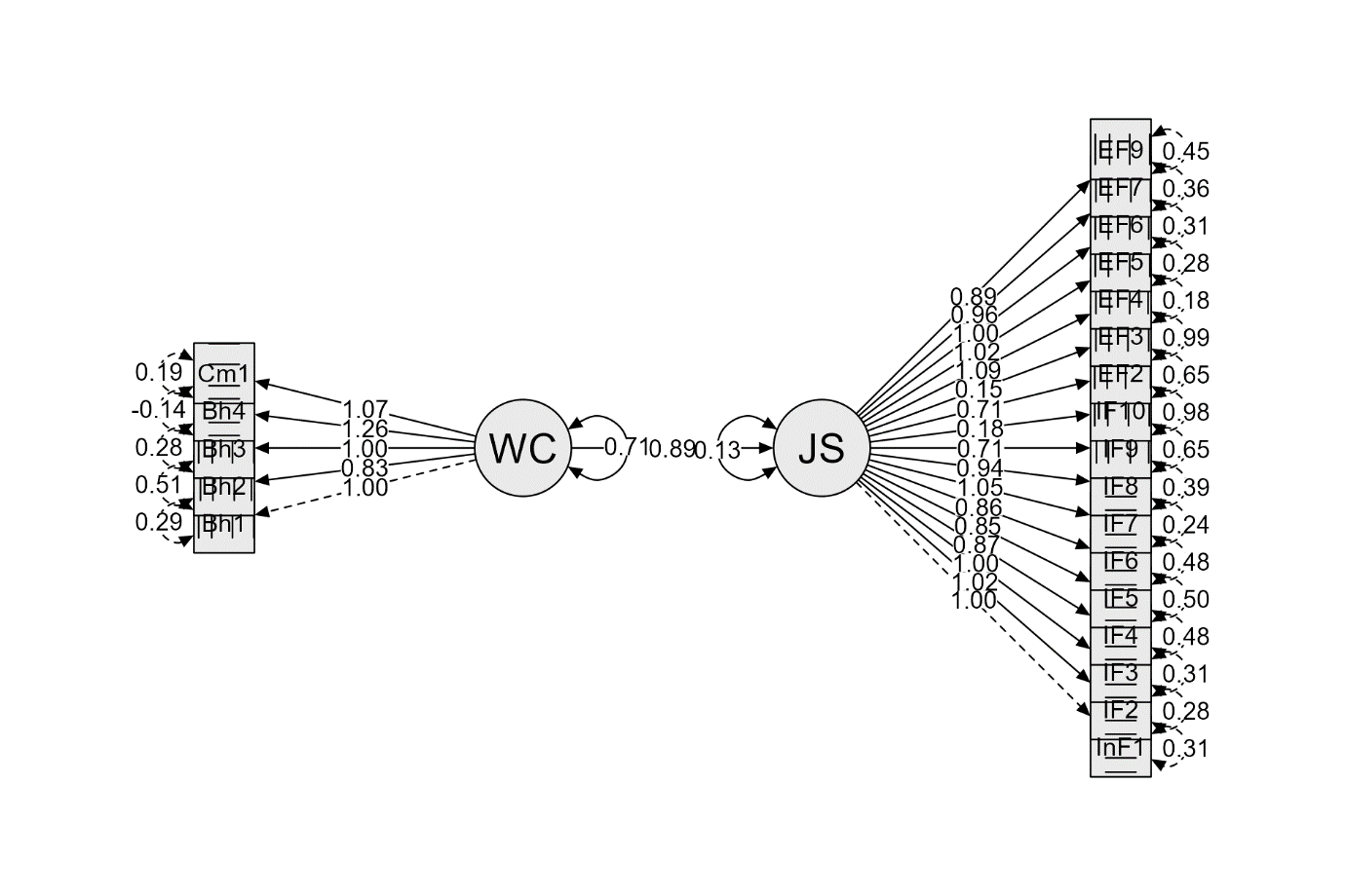
Figure 3. The Path Model |
The Figure 3 above depicts the path model of the variables with their corresponding factor loadings and residual variance values.
CONCLUSION
The hypothesis was satisfied in this research since JASP software was used to run the data for analysis. It is argued that many studies have indicated a more complex situation on job satisfaction in motivating employees which has an impact on productivity and organizational performance (Aziri, 2011). The general objective of this research is to determine the common factors of work culture and job satisfaction that can help bring sustainability to the Metro Mass Transit (MMT) passenger operations. Sinha et al., (2010) argued that the interest that arises in the topic of work culture in this modern times by practitioners and academicians or researchers is been caused by two factors and that is, the first assumption that organizational performance is dependent on the employees’ values are aligned to the extent of the organizations' strategy. And the second aspect is the view that work culture is subject to manipulations consciously to employees’ desired ends. The Metro Mass Transit (MMT) had issues of malpractice, mismanagement of resources, and lack of proper accountability, efficiency, and effectiveness in their service delivery. The model fits and regression coefficients from the JASP results depicted many findings about its application in quantitative research. It can be recommended that future studies can introduce mediation or moderation variables(s) and conduct new research for findings.
ACKNOWLEDGMENTS: I acknowledge that this research solely the authors research aguements and conclusions from the research findings and provided education of JASP withit.
CONFLICT OF INTEREST: None
FINANCIAL SUPPORT: None
ETHICS STATEMENT: None
Agustiningsih, H. N., Thoyib, A., Djumilah, H., & Noermijati, N. (2017). The effect of remuneration, Job satisfaction and OCB on the employee performance. Science Journal of Business and Management, 4(6), 212.
Alnofaiey, Y. H., Almuqati, H. H., Alasmari, A. A., & Aljuaid, R. E. (2022). Level of Knowledge Toward Surgical Site Infections Among Clinical Years Medical Students in the Western Region of Saudi Arabia. Pharmacophore, 13(2), 74-79.
Alzain, H. M., AlJabr, I. A., Al, A. K., Jaafari, H. A. A., AlSubaie, A. S., & Hussein, K. M. (2021). The Impact of Industrial and Community Noise Nuisance on Global Health and Economies. Pharmacophore, 12(3), 64-67.
Aziri, B. (2011). Job satisfaction: A literature review. Management research & practice, 3(4).
Byrne, B. M. (2013). Structural equation modeling with AMOS: Basic concepts, applications, and programming. Routledge.
Cabanas, S., Proença, T., & Carozzo-Todaro, M. (2020). Pay for Individual Performance: Aiding or Harming Sustainable Intrinsic Motivation?. Sustainability, 12(16), 6322.
Cangur, S., & Ercan, I. (2015). Comparison of model fit indices used in structural equation modeling under multivariate normality. Journal of Modern Applied Statistical Methods, 14(1), 152-167.
DeFranzo, S. E. (2011). What’s the difference between qualitative and quantitative research? www.snapsurveys.com accessed 21/04/2023
Dessler, G. (2015). Fundamentals of Human Resource Management, 4th ed. Global Edition. Boston: Pearson International.
Dewi, N. M. (2019). Analisis Pelatihan, OCB (Organizational Citizenship Behavior), Remuneration with Job Satisfaction as an Intervening Variable on Employee Performance. Journal EQ., 6(1), 25031546.
El-Sheikh, A. A., Abonazel, M. R., & Gamil, N. (2017). A review of software packages for structural equation modeling: A comparative study. Applied Mathematics and Physics, 5(3), 85-94. doi:10.12691/amp-5-3-2
Fu, F. Q., Bolander, W., & Jones, E. (2009). Managing the drivers of organizational commitment and salesperson effort: an application of Meyer and Allen’s three components model. Journal of Marketing Theory and Practice, 17(4), 335-350.
Hoelter, J. W. (1983). The Analysis of Covariance Structures Goodness-of-fit Indices. Sociologial Methods and Research, 11(3), 325-344.
Ihinmoyan, T. (2022). Employee Compensation, Retention and Job Satisfaction in Selected Small and Medium Scale Enterprises in Akoko South West Local Government Area Ondo State. Journal of Research in Business and Management, 10(4), 71-76.
JASP Manual. (2018). Seton Hall University, Department of Psychology.
Khojasteh, J. (2012). Investigating the Sensitivity of Goodness-of-fit Indices to Detect Measurement Invariance in the Bifactor Model. Graduate Theses and Dissertations Retrieved from: https://scholarworks.uark.edu/etd/610
Mabaso, C. M., & Dlamini, B. I. (2017). Impact of compensation and benefits on job satisfaction. Research Journal of Business Management, 11(2), 80-90.
Management Study Guide (2019). Work Culture – Meaning, Importance & Characteristics of a Healthy Culture. Officia website, https://www.managementstudyguide.com/work-culture.htm accessed 28th February 2019.
Mulaik, S. A., James, L. R., Van Alstine, J., Bennett, N., Lind, S., & Stilwell, C. D. (1989). Evaluation of goodness-of-fit indices for structural equation models. Psychological Bulletin, 105(3), 430-455.
Navarro, D., Foxcroft, D., & Faulkenberry, T. J. (2019). Learning statistics with JASP: A tutorial for psychology students and other beginners. JASP: Amsterdam, The Netherlands, 418.
O'Malley, A. J., & Neelon, B. H. (2014). Latent factor and latent class models to accommodate heterogeneity, using structural equation. Encyclopedia of Health Economics, 131-140.
Prakoeswa, C. R. S., Endaryanto, A., Martanto, T. W., Wahyuhadi, J., Rochmah, T. N., & Pandin, M. G. R. (2021). Mapping survey of community satisfaction at an academic hospital in Surabaya. The Malaysian Journal of Medical Sciences, 17, 119-122.
Ryan, Richard M., & Deci, E. L. (2017). Self-determination Theory: Basic Psychological Needs in Motivation, Development, and Wellness. New York: Guilford Publications.
Sandika, A. L., Rupasena, L. P., & Abeywickrama, L. M. (2016). Effects of Good Governance Perception towards Job Satisfaction: A Case Study of the Agriculture Professionals Attached to the Department of Agriculture Sri Lanka. Tropical Agricultural Research and Extension, 19(3), 264-273.
Schumacker, R. E., & Lomax, R. G. (2004). A beginners guide to structural equation modelling, 2nd ed. Lawrence Erlbaum Associates, Mahwah.
Shahin, M. (2016). The Effect of Good Governance Mixture in Governmental Organizations on Promotion of Employees’ Job Satisfaction (Case Study: Employees and Faculty Members of Lorestan University). Asian Social Science, 12(5), 108-117. doi:10.5539/ass.v12n5p108
Subramanyam, P., & Donthu, S. (2022). Job satisfaction on job performance of employees in information technology industry. Journal of Contemporary Issues in Business and Government, 28(4), 1135-1147.
Wahyuhadi, J., Hidayah, N., & Aini, Q. (2023). Remuneration, Job Satisfaction, and Performance of Health Workers During the COVID-19 Pandemic Period at the Dr. Soetomo Hospital Surabaya, Indonesia. Psychology Research and Behavior Management, 701-711.
World Bank. (2012). Annual World Bank conference on development economics and governance. Washington, DC: World Bank.
Zayed, N. M., Rashid, M. M., Darwish, S., Faisal-E-Alam, M., Nitsenko, V., & Islam, K. A. (2022). The Power of Compensation System (CS) on Employee Satisfaction (ES): The Mediating Role of Employee Motivation (EM). Economies, 10(11), 290. doi:10.3390/economies10110290