INTRODUCTION

Stock return is one of the most important indicators used to measure the activities of a firm. The stock return is a theme that has been formed based on the quantitative expansion techniques of financial management and assessment of needs of financial statement users. Therefore, stock return is beyond the measurement of past activities and enables financial managers to help decision-makers (saidi, 2021).

On the other hand, factors affecting the stock return are crucial factors in investment decisions. Researchers and scientists of decision-making and prediction need to select the variables affecting the outcome of decisions and forecasts Hence, many studies support the role of macroeconomic factors in determining stock return (Madani & Tajvidi, 2020; Jaghoubi, 2021). However, the fundamental mechanism in which macroeconomic factors, monetary and financial shocks, and stock return are interconnected factors has not been solved as a theoretical problem.

Actualization of macroeconomic goals, such as output growth and inflation control along with increased investment and employment, are substantial subjects of the economic policies of every country. Since monetary and financial policies are the most important economic means used to achieve the aforementioned goals, many studies have examined the effectiveness of such policies. On the other hand, monetary and financial shocks may lead to booms and busts (Dargahi & Hadian, 2016).

In terms of monetary shocks under the theoretical framework, economists have a consensus on money neutrality within the long term, i.e., monetary shocks do not cause a permanent change in the real sector of the economy. However, there are some disagreements on the short-run effects of monetary shocks. According to some theories, monetary policies and shocks have real short-run effects on the economy, while others believe in neutral short-run effects of monetary policies (Brooks, 2007).

The role of monetary and financial shocks in economic growth has been highly considered over recent years regarding the effect of predicted and unpredicted (shocks) factors and the asymmetric impact of these shocks. In this case, empirical studies of Ahmad, (2019) indicated the negative effect of monetary and financial shocks on the economic growth of studied countries. In an accurate review, results of empirical studies conducted by Karas et al. 2013 found the negative effect of financial and monetary shocks on the economic growth of developed countries, while this effect was positive in developing countries. However, Santiago et al., (2020) and found no significant relationship between economic growth and government expenditure shock in the studied countries. 

It is vital for stakeholders and economic actors to identify the effects of monetary and financial on the stock return, particularly in the stock exchange market. Hence, the effect of financial and monetary shocks on stock return can be found through the field and scientific studies. Therefore, the lack of such study on financial management is a research gap, and the extant study aims to fill this gap by answering the following questions based on scientific methods: do monetary shocks have a positive and significant effect on the stock return?  Do financial shocks have a positive and significant effect on the stock return?

Literature Review

Monetary Shocks

Monetary shock is a process in which monetary authorities of a country control the money supply to adjust interest rates regarding economic growth, sustainability, relative price stability, and lower unemployment. There are usually two contractionary and expansionary monetary shocks, in which the money supply is set to achieve specific goals under different conditions. In general, monetary policy is a part of economic policies through which monetary authorities try to control the money supply in line with other economic policies to achieve economic goals (Farooji & Amir Jabbari, 2016). Quantitative instruments of monetary policy are as follows:

Legal Reserve Ratio (LRR)

LRR is the only variable in the money multiplier that is under the control of the central bank. This monetary instrument concerns changes in reserves that commercial banks are legally binding to keep in the central bank with or without interest. LRR is the legal parameter of the aforementioned action. The central bank can use this monetary instrument based on the case and monetary-economic situation of the country changing LRRs affecting LRRs and the lending capacity of commercial banks (Abedi & Setoodehnia, 2013). The use of certain monetary instruments to achieve determined goals and monetary policies includes a set of decisions and measures taken to control money volume and credit by the central bank. In this case, the central bank affects the expenditure flow and fulfills the economic goals by changing the money supply and interest rate.

Rediscount Rate

Commercial banks can rediscount the authenticated promissory notes of customers (who have discounted those notes in the commercial banks) in the central bank to provide financial resources. The central bank is allowed to apply the monetary policy in this way, which is called the rediscount instrument.

Open Market Operation (OMO)

The central bank usually buys or sells different types of government bonds to use open market operations and apply monetary policies. The governmental bonds are usually long-run with fixed interest rates relative to their nominal values. The operational parameter of monetary policy is determined through open market operations. On the other hand, the central bank determines the quantity of selling or buying these bonds in the market. Therefore, the effective application of OMO as an instrument to control the monetary base depends on an extensive market for governmental bonds. Since such a market does not exist in developing countries, only developed countries use OMO (KUSUMATRISN, 2022).

The qualitative monetary instruments provide the central bank with a set of instruments that monetary authorities can use to affect the money consumption in the economy, i.e., monetary authorities use these instruments to allocate bank credits to economic sectors and determine the consumption share of each economic sector in the whole credits. Qualitative monetary instruments are preferable since quantitative instruments cannot make a difference between economic sectors in terms of granting credits. However, in specific economic conditions that require different monetary policies to control or grant credits in different economic sectors, qualitative monetary instruments leave the highest economic effects. The qualitative instruments include total credits, selective credit controls, interest rate regulations, and moral suasion.

Financial Shocks

Financial shock means government impulse originated from government purchases, transition payments, and tax structure. In economics and political sciences, financial shock uses two instruments of government income (tax) and expenditure (cost) to affect the economy. Financial shock usually includes three types:

Expansionary financial shock: expansionary fiscal policy is selected under the lack of full employment while there is an economic and market recession. This policy includes increasing government expenditure and reducing taxes to expand economic activity and fill the contractionary gap.

Contractionary financial shock: this impulse is selected when there is high employment and inflation caused by excessive exploitation of production resources. Contractionary financial shock is used to reduce demand pressure and inflation, and fill the inflationary gap by increasing taxes and reducing government expenditure.

Neutral financial shock: this impulse is imposed in the case of economic equilibrium. Government expenditure is provisioned by tax incomes so that the budget leaves a neutral effect on economic activities (Hashemi Dizaj, 2012).

The Relationship Between Financial-Monetary Shocks and Stock Return

Tobin (1969) designed a model based on his general equilibrium theory indicating that both monetary and financial shocks had significant effects on return on assets (ROA). According to this approach, fiscal events and shocks affect the aggregate demand by changing the valuation of physical assets related to their substitution costs. It must be noted that an increase in money supply or reduction in interest rate leads to higher demand for stock; therefore, the stock price will increase that, in turn, increases investment expenditure and aggregate demand (Boivin & Giannoni, 2002). In other words, an increased nominal interest rate leads to an increase in the cost of capital use and a decline in investment and consumption costs reducing the real activity of the economy.

Moreover, increased money supply leads to higher cash available for individuals than their optimal inventory. Hence, individuals spend their surplus cash to buy goods, services, and other financial assets, such as stock. Increased demand for stock leads to higher prices and return of the stock. The other theories, including Fisher's portfolio theory, explain the effects of monetary and financial shocks on the return on assets. Furthermore, the association between financial-monetary shocks and stock return can be examined theoretically by generalizing the theory of the portfolio model of Brunner and Cagan In general, expansionary fiscal policy contributes to higher production and economic growth, helping the government to implement its plans by spending costs on the development of infrastructural sectors, such as highways, water, and sewage systems, transportation, power, etc. that lead to increased output and economic growth in the long term. In this case, the government can stimulate private investment by developing foreign savings.

Studied the relationship0 between stock return predictability and variable inflation level. Arajollahi & Asgharpour, (2019) examined the effect of change in money supply on liquidity and share price. Their results showed a positive effect of money supply change on liquidity. On the other hand, after controls for monetary regime switches and the Global Financial Crisis, liquidity change had a positive effect on the share price. These findings, obtained after solutions to several econometric deficiencies in prior studies, provide clear verification of the endogenous money supply theory, money effect on liquidity, and the extension of the model for a liquidity effect on asset prices. Malik, (2013) examined the effect of fiscal shocks on the performance of monetary policy rules in a dynamic general equilibrium framework. Their analysis suggested that some form of flexible inflation targeting regime would perform well in response to fiscal shocks compared to other forms of policy regimes. Kim and Rescigno, (2017) studied the relationship between expansionary monetary shock and increased firm's return and found that expansionary monetary shocks disproportionately increased returns of a distressed firm, which had profit substantially smaller than its interest expense and required external financing.

Table 1. Summary of results of previous studies

Impulse Response Function

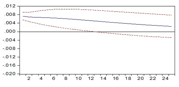
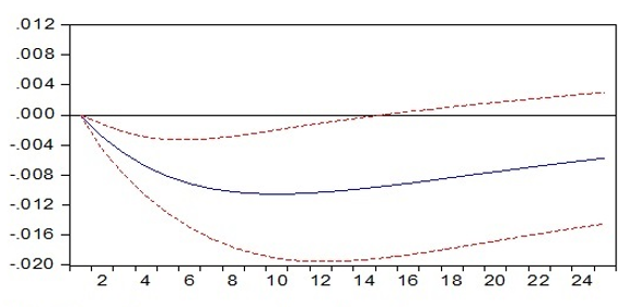
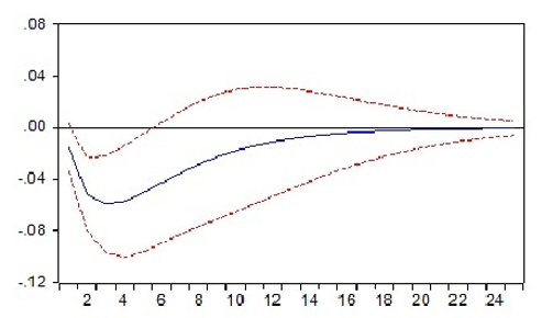
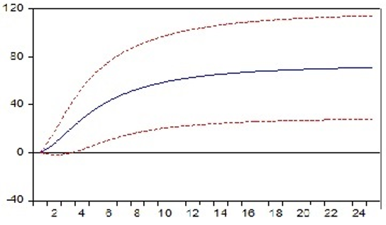
As stated, these functions reveal the response of the dependent variable in the model to the shock inflicted on other variables. Shock analysis shows two key points: one is the significance of the shock effect and the other is its effect damping in the long run that indicates the model’s stationarity. Below are diagrams derived from the impulse-response functions. The extracted tables are also provided in the appendices.  Looking at diagrams 1 to 4, it is noted that liquidity shock has a positive and significant impact on the stock return index for 13 periods, thus, resulting in shock damping. Moreover, the shock

 from the government’s spending on production will leave a negative and significant impact on the stocks to return index for 13 periods, thus resulting in the shock damping. The inflationary shock will have a negative and significant impact on the index for 5 periods.  

Analysis of Variance results

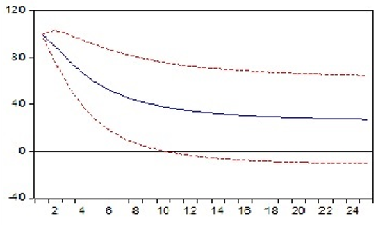
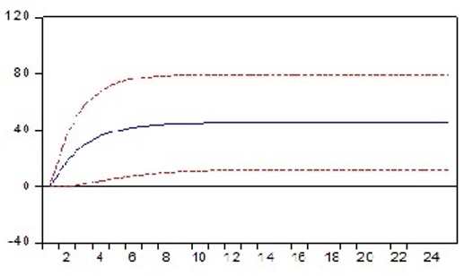
As stated, the prediction error analysis of variance method is one of the applications of the vector auto-regressive models, which examines the contribution of each exogenous variable to the shock inflicted on the dependent variable. Using this method, it is learned to what extent the variations of a variable may be affected by the error terms of the variable itself, and also affected by error terms of other variables inside the system.

Looking at the appendix table and diagrams 5 to 8, it is noted that in the long run, 28% of the prediction error variance of the stocks return index was attributed to the index shock itself while being insignificant; however, 70% of which is attributed to the government’s spendings shock to the production. Fifty-one percent of the prediction error variance of the index is explained by the liquidity growth. Also, 46% of this error is attributed to the inflation shock.

MATERIALS AND METHODS

The extant study was applied in terms of objective and was descriptive in terms of method. The data were collected from organizational information and reports published by companies listed in the stock market by using audited financial statements of the firms listed on the official website of Tehran Stock Market and Rahavard Novin software. The statistical population comprised companies listed in Tehran Stock Market during 1983-2016. The research variables were assessed in this way:

To calculate the return rate of ordinary stock, the price of the ordinary stock at the end of the fiscal year was subtracted from its price in the early days of the same year, then receivable dividends were added, and the outcome was divided by the total price of that share in the early stage of the period

End-of-period value is defined as the share value after applying modifications of capital rise plus the dividends per share; initial value is the stock price at the beginning of the period

In this research, liquidity was used as the monetary shock index, while government expenditure represented the financial shock index. The simplest vector autoregression (VAR) model includes two variables.

The first step to the VAR model is determining the optimal lag of the model. Two common criteria are used to determine optimal lag: Akaike Information Criterion (AIC) and Schwartz Bayesian Criterion (SBC).

One way to examine the causal relationship between variables is by testing the lags of a variable in the equation of another variable. In a model with two equations and p lags, (yt ) will not be the Granger causality of (zt ) if and only if all coefficients of A21(L)  equal zero. In other words, (yt ) will not be the Granger causality of (zt ) if (yt ) cannot increase the prediction power of (zt ). F all variables in the VAR model are stationary, the direct method of the Granger causality test is the use of the standard F value for testing the constraint below:  

The equation (3) can be generalized to the n-variable model. Since Aij(L)  represents delayed coefficients of variable j in the equation of variable i; if all polynomial coefficients of Aij(L)  equal zero, variable j will not be the Granger causality of variable i.

Hypotheses

Hypothesis 1: Monetary shocks have a positive and significant effect on stock return.

Hypothesis 2: Financial shocks have a negative and significant effect on stock return.

Findings

According to the Augmented Dickey-Fuller test, all variables were stationary at level. Table 2 reports the summary of the results.

Table 2. Summary of results of previous studies

After the initial VAR model was estimated, the optimal lag was selected based on the considered criteria. Table 3 reports the respective results.

Table 3. Determining the optimal lag of the model

According to the research topic and variables introduced in the model, the stock return index was estimated based on the VAR structure shown below: 

The vector of endogenous variables is shown for the model:

Model: examining stock return index: Investigating the stock return index with regard to the relationship between stock return (LNSR) and government spending to production (g) and the growth of liquidity to production (rm) and inflation (inf).

P indicates the degree of estimated VAR or number of inserted lags of endogenous variables that are calculated based on the optimal lag criteria.

According to the time-series of variables, two dummy variables of 1986 and 2008 were entered as endogenous and control variables in the estimation step. The dummy variable of 1986 was associated with severe output decline shock and economic recession (due to reduced oil revenues in 1985), and the dummy variable of 2008 was associated with government expenditure growth and change in the interest rate of bank deposits.

Table 4. Granger causality of model

According to Table 4, Granger rejected the null hypothesis of all variables; therefore, all variables were Granger causality of stock return index. Accordingly, government expenditure was causality f stock return index at the confidence level of 99%. Liquidity could be a causality of the stock return index at the confidence level of 99%, and inflation could be taken into account the causality of the stock return index at the confidence level of 99%.

The impulse response functions have been illustrated in Figures 1a-1d. According to these diagrams, liquidity shock had a positive and significant effect on the stock return index for 13 periods; then, the shock effect is dampened. Moreover, government expenditure shock to production had a negative and significant effect on the stock return index for 13 periods, and then the effect was lost. The inflation shock also had a negative and significant effect on the index for five periods.

According to Figures 2a-2d, 28% of the prediction error variance of the stock return index was attributed to the stock return index's shock, but it was insignificant, while its 70% was attributed to government expenditure shock to the production. Moreover, 51% of the prediction error variance of the index was explained by liquidity growth, and 46% of this error was attributed to the inflation shock. 

CONCLUSION

The purpose of the extant study was to examine and compare financial and monetary shock on the stock return in the stock exchange market. According to the Granger casualty test, liquidity was taken into account as the cause of stock return at the confidence level of 99%. The dynamic analysis indicated the positive and significant effect of liquidity shock on the stock return over 13 periods, and then the effect was dampened. This variable also could explain 51% of prediction error variance in the long term. In terms of the positive relationship between the stock market and money supply, it can be explained that money affects the stock price index within two dimensions; first, it is an effective macroeconomic variable, and second, this variable is considered an asset in investor's portfolio. Moreover, variations in money supply are a factor affecting the important economic variable, so that money supply can play a vital role in achieving the economic goals of a country, such as capital market growth and development. Hence, the relationship between the money supply and the overall stock market index must be positive theoretically. This positive effect occurs due to some reasons: firstly, increased liquidity can increase the demand for assets, such as stock; secondly, expansionary monetary policy in Iran's economy leaves positive mental effects on expectations and desire for investment, paving the way for the positive relationship between the stock market index and money supply.

According to the Granger casualty test, government expenditure was taken into account as the cause of stock return at the confidence level of 99%. The dynamic analysis indicated the negative and significant effect of government expenditure shock on the stock return over 13 periods, and then the effect was dampened. This variable also could explain 70% of prediction error variance in the long term. In terms of the negative relationship between the stock market index and government expenditure, it can be explained that after the Revolution in Iran, the government used credits from the central bank and commercial banks to provide a budget deficit that led to increased liquidity. Since the increased liquidity was not used in productive sectors, this increased rate led to inflation, and a higher inflation rate led to a higher interest rate. The higher interest rate, in turn, increased the expected return rate of investors, which is used as the discount rate to determine the value of financial assets. Therefore, the increased return rate of investors leads to a reduction in the present value of future earnings and a decline in stock value and the stock market. On the other hand, the effect of a negative increased government expenditure shock on the Iranian stock market indicates the inefficiency of the private sector because when the government's budget deficit is supported through borrowing from the central bank or even commercial bank, the inflation rate is increased and private sector cannot work freely. The aforementioned reasons intensify the inefficiency of the private sector.

The obtained results indicated the positive effect of the shock of increased liquidity on Iran's stock market; hence, the monetary policy-caused shock had a positive effect on the stock market of Iran. Therefore, increased liquidity leads to an increase in the stock market index. However, the shock caused by increased government expenditure had a negative effect on Iran's stock market. Hence, the financial policy-induced shock had a negative effect on the stock market and reduced its index. Accordingly, increased government expenditure reduced the stock market index.

According to the results of the present paper, it is suggested that policymakers pay attention to the conditions of the stock market by applying monetary and fiscal policies. It is recommended that investors consider the economic conditions, particularly monetary and fiscal policies made during their investment periods. Investors can make accurate investment decisions by obtaining detailed and up-to-date information about investment decisions.

ACKNOWLEDGMENTS: None

CONFLICT OF INTEREST: None

FINANCIAL SUPPORT: None

ETHICS STATEMENT: None